Correlation is not always what it seems - an often overlooked aspect in time series analysis2/5/2014
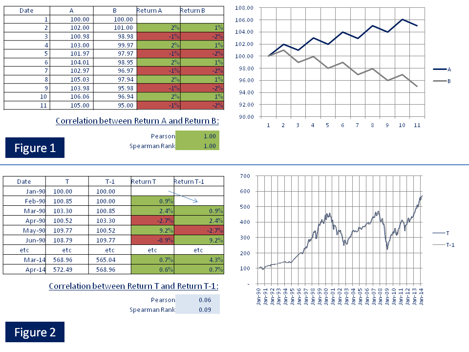
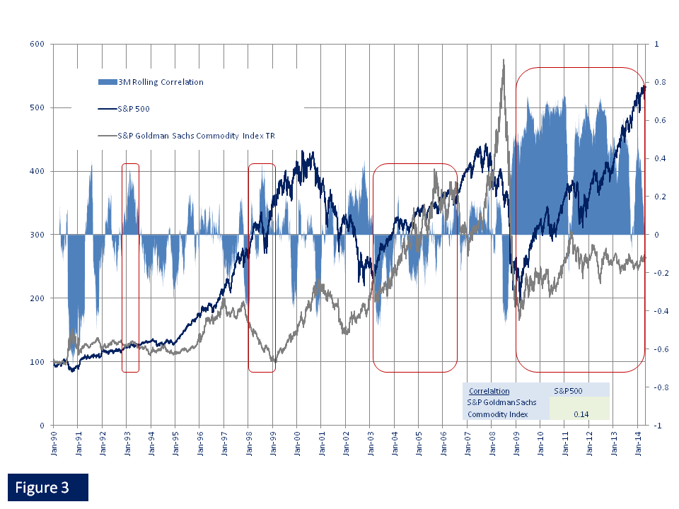
Abstract Many CTAs and other money managers use correlation in time series analysis in their daily work to derive investment decisions on asset allocation, risk and money management, tactical overlays, or selection of products or markets. In J8, we do not use correlation as input parameter in our design to achieve diversification benefits or to derive investment decisions thereupon. We focus our efforts on sound return generation of the single underlying asset. We then enjoy diversification benefits that may come into play naturally when we put different asset classes and trading models together into a portfolio. Why we dislike correlation analysis We refrain from using correlation analysis in our money management and strategy designs mainly for two reasons: a) historical correlations between assets may dramatically and long lastingly change under unexpected new market conditions, rendering any predictive power ascribed to future expected returns derived from past returns and correlations, worthless; and b) looking at the correlation coefficient alone for describing the relationship between two assets may fool you greatly about the true nature of their relationship. Hypothetical examples 1 & 2 The correlation coefficient in Table 1a for the hypothetical time series A and B in Table 1 and Figure 1 is r=1. This suggests that return series A and B are perfectly correlated with each other and should move in log-step. In reality, however, they drift in opposite directions and hedging exposure to A by using B will cost a lot of money in the long term. It is not a good hedge even though a correlation of r=1 may suggest so. In converse, in Table 2, 2a and Figure 2, we used the monthly returns of the S&P 500 for time series "T" and created a new hypothetical time series using the same S&P 500 returns, but shifting the time series by one month, and call the new series "T-1". Both time series move almost in perfect sync over the years. However, the correlation coefficient of r=0 between both series T and T-1 suggests total independence of both assets and conventional wisdom tells us they are not good for hedging each other. In reality, however, they drift in the same direction and using asset T-1 to hedge asset T in the long-term may prove to be useful. It might be a good hedge even though a correlation of r=0 does not suggest so. Note: Past performance is not indicative for future performance. Source: J8 Capital Management LLP, Bloomberg LP. Real example 3 We now test if our observations from the hypothetical examples hold in the real world. For this, we take a look at the correlation between the S&P 500 and the S&P Goldman Sachs Commodity Index Total Return from 1990 until today. Table 3 shows both asset classes to be uncorrelated, or lightly positively correlated.Now, in Figure 3, we take a closer look and plot the time series for both assets together with their three months rolling correlation. We make following broad and generalizing real world observations, confirming our observations from the hypothetical examples: - Regime shift: while the sign of the correlations changed frequently form the early 1990s until the financial crisis in 2008, since 2009 the regime has shifted into a highly positive correlated relationship. - 1998: commodities trend down, equities trend up, and the correlation is positive - 2003 until mid 2006: Both trend up with average correlation negative It appears to be very difficult, if not impossible, to base predictions of future return developments between two asset classes on their historical relationships. Discussion and outlook
The correlation coefficient merely captures the linear relationship between two return series. Even if for example the relationship between A and B in example 1, was not exact, the magnitude of the correlation coefficient would still not be helpful for successful hedging purposes. One may intuitively suggest "let's do beta hedging", which is in essence the use of a multiplier to describe a linear regressed relationship between two return series. Also here, our reason a) for disliking correlation in the first place, kicks in. We discard such approaches for designing robust trading systems, because again, historical relationships between different assets may not hold for the future. Example 3 illustrates the problem of using historical correlations for future predictions. The above examples 1 & 2 are constructed and hypothetical. They demonstrate a general problem we encountered when considering using correlations to derive investment decisions. In particular the examples demonstrate the danger of relying on historical performance for future investment decisions and strongly support arguments against its use. Some academics suggest looking at trends within the data series as additional information to the correlation coefficient. This, however, may open yet again a Pandora's Box of flaws associated with trend following systems and introduce additional uncertainty. Conclusion Conventional measures of correlation tell us only part of the relationship between the return series of two assets. Also, historical relationships may not hold for the future. Using correlations as building blocks in a trading system therefore may introduces further uncertainty. We abstain from using correlation in our model design or management decisions.
7 Comments
|
- About
- J8 GARS
- Regulatory Hosting
-
Research
- J8 CTA Index
- Videos >
- JII - A liquid and investible benchmark index for the CTA and MF industry
- THFJ - Common Denominators in CTAs: Traded Markets
- THFJ - Common Denominators in CTAs: Portfolio Construction and Index
- JII - Common denominators in the CTA and managed futures industry: A survey report
- THFJ - Correlation is not always what it seems
- Quantifying Political Risks - PhD Thesis
- Contact
|
PRUDENT investment management.
|
PROCESS driven strategy.
|
PERSISTENCE in returns.
|
|
J8 Capital Management LLP is authorised and regulated by the Financial Conduct Authority in the United Kingdom
J8 Capital Management LLP is registerred with the National Futures Association in the United States. |
J8 Capital Management LLP (c) copyright 2024
|


 RSS Feed